By Shivani Garg
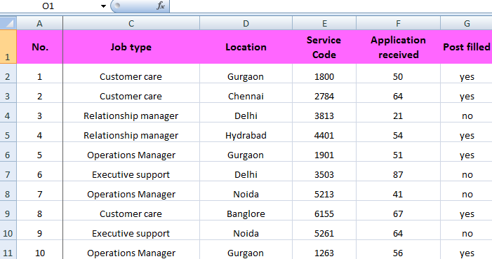
When you work with lot of data, it can be difficult to keep look on complete data in worksheet. It happens a lot of times that when you scroll down the worksheet, You are unable to see the headings in Top row. At this time it can useful to freeze rows or columns.
MS Excel makes it easier to view data from different ends of your worksheet at same time by using the feature Freeze panes.
How to Freeze Top Row of Worksheet in MS Excel
Let's learn with Example
>> Click View Tab and then click Freeze Panes.

>> Click Freeze Top Row.

>> Now you can scroll down the worksheet. You will see that top row is frozen and this is indicated by dark grey horizontal line under top row.

How to Freeze First column of Worksheet in MS Excel
Let's learn with Example
>> Click View Tab and then click Freeze Panes.
>> Click Freeze First Column.

>> Now you can scroll the worksheet. You will see that First Column is frozen and this is indicated by dark grey horizontal after First column.
How to Freeze Panes of Worksheet in MS Excel
Let's learn with Example
>> Select the Row from where you want to freeze panes. For example, Let's select Row 5 here.
>> Click View Tab and then click Freeze Panes.
>> Click Freeze Panes.

>> Scroll down the worksheet and the result will be above rows are frozen

In the same way Column can be frozen. You just have to select column instead of Rows while freezing column
How to Unfreeze Panes of Worksheet in MS Excel
Let's learn with Example
>> Click View Tab and then click Freeze Panes.
>> Click Unfreeze Panes.

Result will be

** You cannot freeze panes and split panes at the same time. You can enable only one of the two.
Also read : MS Excel tutorials for you :)
Related >>
Labels:
MS Excel
Shivani Garg